How To Use Vlookup In Microsoft Excel And Google Sheets

You can do a lot in Microsoft Excel and Google Sheets, beyond the obvious spreadsheet-style organization and data collating. A lot of this is tied to both of their programming-like functions that can be used to automatically tally totals, organize rows or columns for you, and so on.
The VLOOKUP function offers a similar kind of spreadsheet help, though it's main purpose is for digging up specific details within a defined range. Particularly useful with very large spreadsheets with a wide variety of data points. For example, if you're keeping track of pin or sticker sales you can use VLOOKUP to search a given column (on-hand quantities, sales numbers, pricing, etc) and return only the value you want to look up (such as pricing for stickers, pricing for pins, etc). And once you've set up the function, you can reuse it to search for other data points in the designated cell range without much hassle. Or even create multiple VLOOKUP cells that each check a different column in the cell range so you can look up other values without adjusting the function code.
Much like other functions, however, the trick to using VLOOKUP effectively is knowing what commands and values to use in what order. Again, much like programming languages. Though in this instance the formula is the same between both Excel and Sheets, so you can use the same technique for either of them interchangeably.
VLOOKUP in Excel and Sheets
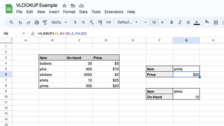
When you're ready to start searching, here's what you do:
- In Excel or Sheets, select an empty cell and type the name (or item number, etc) of what you want to search for. Let's call this the Named Cell.
- Select a cell directly below or next to the Named Cell (location isn't essential but keeping it close makes finding results easier) and type "=VLOOKUP" to pull up a small VLOOKUP function window.
- Click on the Named Cell (this will add it to the VLOOKUP function), then press the comma (,) key.
- Now click the first cell in the top-left most area of the range you want to search, then click the last cell in the bottom-right most area of the desired cell range and press the comma (,) key. This is the area VLOOKUP will search.
- Enter a number to designate the column within the cell range you want to search (ex: the tenth would be is "10")
- Press Enter or Return (for Windows or Mac, respectively) to close the function window.
- Or, after entering the last number press the comma (,) key and type in "FALSE" to tell VLOOKUP to only provide exact matches rather than approximate ones. Then hit Enter or Return to finish.
VLOOKUP will display the search results in the cell the function was entered into, and you can change the text in the Named Cell to search for other items in the designated cell range as much as you need.