How To Freeze A Row In Microsoft Excel And Google Sheets

When you're working on an especially chunky spreadsheet in Microsoft Excel or Google Sheets, it can get annoying to have to scroll up, down, and around to keep track of where all the information is supposed to be going. This bit goes in this column, and that bit goes in that row, but only if it's under this specific such-and-such. It's an absolute headache, especially if you're trying to remember a bunch of things at once, and it falls out of your head by the time you scroll back to where you were.
Thankfully, Excel and Sheets have a feature to alleviate this burden a bit. Instead of needing to scroll back to the top of your document to check things, you can freeze rows and columns, keeping them pinned on the sheet as you work so you can consult them at a moment's notice. Freezing rows is quick and easy, certainly more so than all that scrolling.
How to freeze a row or column in Microsoft Excel
The freezing function has been available in Microsoft Excel for well over a decade now, allowing you to pin rows and columns to your view as you work. While the method we're about to outline is intended to work with the modern version of Excel, you can freeze rows in older Excel versions roughly the same way.
- Open a spreadsheet in Microsoft Excel.
- Switch to the View tab in the top taskbar.
- On the right side of the View menu, you'll see three Freeze buttons.
- Click Freeze Panes to freeze everything to the left of your currently-selected cell.
- Click Freeze Top Row to freeze the topmost row of the spreadsheet.
- Click Freeze First Column to freeze the leftmost column of the spreadsheet.
- While Freezing is active, Freeze Panes becomes Unfreeze Panes.
To elaborate a bit further on Freeze Panes, when clicked, the button creates a kind of "reticle" at the cell you currently have highlighted. Everything above and to the left of this cell will be frozen while the rest of the spreadsheet scrolls as usual. So, for example, if you freeze at cell H10, every cell from A1 to G9 will be pinned. Whatever freeze function you use, you can disable it at any time by clicking the Unfreeze Panes button.
How to freeze a row or column in Google Sheets
Google Sheets' freezing function allows you to pin not just the topmost row and leftmost column to your view but even create larger, more specific freeze-frames based on your preferences. You can freeze all but one cell if you feel so inclined, though that might make it a bit difficult to work.
- Open a spreadsheet in Google Sheets.
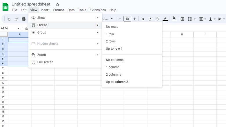
- Click the View button in the top taskbar.
- Select Freeze.
- Click 1 row to freeze the top row, 2 rows to freeze the top two rows, or Up to row (X) to freeze every row up to your currently-selected cell.
- Alternatively, click 1 column to freeze the leftmost column, 2 columns to freeze the two leftmost columns, or Up to Column (X) to freeze every column up to your currently-selected cell.
- Click No rows or No columns to unfreeze your currently-frozen rows and columns, respectively.
By using the two "Up to" options, you can create a cross-pattern of frozen rows and columns to keep more of the spreadsheet in your view as you scroll.